Translation of texts contained in Excel formulae

Dear Community!

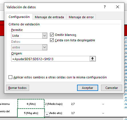
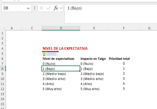
I need help with the settings of an excel containing the following formulae:

Excel screenshot showing a formula bar with a nested IF statement and cells with '#VALUE!' errors in columns 'Probabilidad' and 'Impacto en Talgo'.

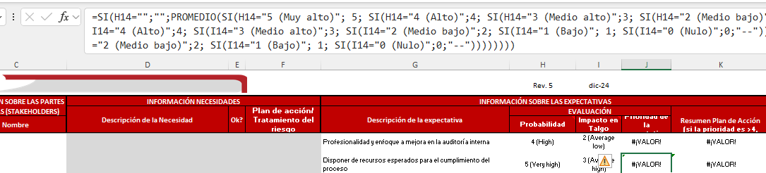
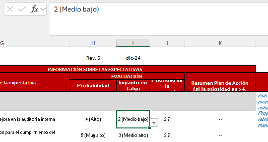
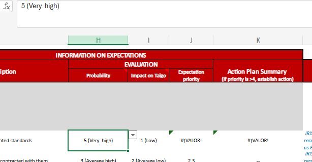
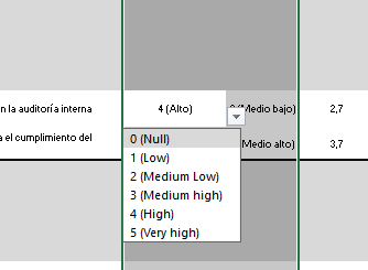
I have translated the texts in Columns "Probabilidad" and "Impacto en Talgo", replacing them with "High " and "Very high", however, as you can see, the referenced values in the two Columns on the right show an error.

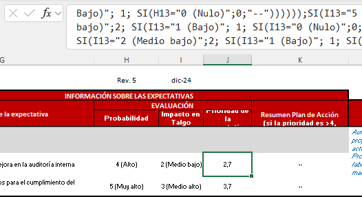
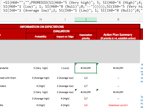
Above, you can see the formula, containing the same parameters (high, low, etc.).They are not translated and this is what causes the errors.

Any idea on how to make this embedded content visible in Trados and avoid the error? Seems like it is impossible to do it manually. 

Thanks in advance!

emoji
Parents
  •   

    I don’t think you can extract Excel formulas in Trados. So you can only prepare better the spread-sheet.

    Are cells in columns H and I picked from a list somewhere else? If so, you can edit the formula to pick those values. For example, if the list of values shown in column H is in a separate sheet called Values, and in the range A2:A7, you’ll need to replace:

    H14="5 (Muy Alto)"

    with:

    H14=Values!A$2

    in the formula of cell J14. You'll need to edit the remaining IF and a similar thing in the cell above. At the end of the replacements, you won’t have strings inside the SI functions and it should work. If you only have to edit a couple of cells, this edition is feasible, otherwise, it can be a real pain to prepare...

    Good luck!

    emoji
  • Thank you,   and  :

    let me be more specific. 

    Screenshots 1 and 2 (before): original document. The selected cell IS extracted by Trados as text and can be translated:

    Screenshot of a spreadsheet with cells showing text in Spanish, no visible errors.

    However, in the next column there is a numerical value (calculation result). The formula is:

    Spreadsheet with a formula bar displaying a complex formula in Spanish, no errors visible.

    Screenshots 3 and 4 (after): Once translated (columns H and I), the resuls in column J and K show errors:

    Spreadsheet after translation showing '#VALUE!' errors in columns J and K for 'Expectation priority'.

    Columns H and I were translated in Trados.

    Spreadsheet with formula bar in English showing '#VALUE!' errors in cells and a note 'Establish action!' in column K.

    And this is the result after the replacement of the texts in the formula manually (with Search and Replace function)

    So,  , I did not understand, what should be replaced with the combinations you mentioned in your answer...but I hope that the issue is clearer now , with these screenshots.

    Many, many thanks in advance!

    emoji


    Generated Image Alt-Text
    [edited by: RWS Community AI at 8:26 AM (GMT 0) on 27 Feb 2025]
  •  

    I mentioned lookup table in my response and the screenshot you have shown looks to be just that.  Note the dropdown arrow in this cell:

    Screenshot showing a dropdown menu with the selected option '5 (Very High)' and a red arrow pointing to the dropdown arrow.

    That should tell you that these values are drawn from a list, possibly on a different worksheet (might even be hidden), and it is the values in that location that you should be translating, and not the ones in column H and I.

    You really need to understand how the original spreadsheet is working and only then will you be able to understand the true nature of the problem... from your screenshots we can only guess.

    Paul Filkin | RWS Group

    ________________________
    Design your own training!

    You've done the courses and still need to go a little further, or still not clear? 
    Tell us what you need in our Community Solutions Hub

    emoji


    Generated Image Alt-Text
    [edited by: RWS Community AI at 8:45 AM (GMT 0) on 27 Feb 2025]
  • You are absolutely right, Paul! There is a dropdown list, so I have to find the elements of the list....but this is the only thing I can get to:

    Screenshot of a 'Validacion de datos' (Data Validation) dialog box with settings for a dropdown list in a spreadsheet application. An error message or list is not visible.

    I cannot see the list though....

    emoji


    Generated Image Alt-Text
    [edited by: RWS Community AI at 9:25 AM (GMT 0) on 27 Feb 2025]
  •   

    You need to go to the sheet Ayuda. Then the range where the values are picked-up is D7:13

    The replacements mentioned in my post need to point to the values in this range.

    emoji
  • I have just done it...but these are already translated, looks like Trados detected them as text.

    Screenshot of a spreadsheet with a selected cell D8 containing the text '1 (Bajo)'. Columns titled 'Nivel de expectativas', 'Impacto en Talgo', and 'Prioridad total' with corresponding rows ranging from 0 (Nulo) to 5 (Muy alto).

    So...what is here to replace?? This is the original doc (the target one has these words in English...)

    emoji


    Generated Image Alt-Text
    [edited by: RWS Community AI at 9:35 AM (GMT 0) on 27 Feb 2025]
  •  

    Can you provide the complete formula used in the cell that errors?  You want quite detailed help but don't provide enough information to help so we probably spend a lot more time guessing than is really needed here.

    A sample spreadsheet would be even better.  If you deleted everything apart from a couple of rows, and anonymized any text, then that would surely help!

    Paul Filkin | RWS Group

    ________________________
    Design your own training!

    You've done the courses and still need to go a little further, or still not clear? 
    Tell us what you need in our Community Solutions Hub

    emoji
  • You are right, Paul! I have prepared the file:

    7870.Sample excel (tab 3).xlsx

    *Establecer acción is in herited from the original file (does not require fixing)

    Thank you so much!!!

    emoji
  •  

    I didn't really understand this comment:

    *Establecer acción is in herited from the original file (does not require fixing)

    But I did manage to get rid of the error... but I have some questions over the result because I could not test exactly what you had since I have an English version and the syntax is a  bit different (SI vs IF etc.).  But essentially, I translated the values in the Ayuda worksheet only, then replaced this:

    =IF(H13="","",AVERAGE(IF(H13="5 (Muy alto)", 5, IF(H13="4 (Alto)",4, IF(H13="3 (Medio alto)",3, IF(H13="2 (Medio bajo)",2, IF(H13="1 (Bajo)", 1, IF(H13="0 (Nulo)",0,"--")))))),IF(I13="5 (Muy alto)", 5, IF(I13="4 (Alto)",4, IF(I13="3 (Medio alto)",3, IF(I13="2 (Medio bajo)",2, IF(I13="1 (Bajo)", 1, IF(I13="0 (Nulo)",0,"--")))))), IF(I13="5 (Muy alto)", 5, IF(I13="4 (Alto)",4, IF(I13="3 (Medio alto)",3, IF(I13="2 (Medio bajo)",2, IF(I13="1 (Bajo)", 1, IF(I13="0 (Nulo)",0,"--"))))))))

    With this:

    =IF(AND(H13<>"", I13<>"", J13<>""), AVERAGE(IF(H13="5 (Very high)",5,IF(H13="4 (High)",4,IF(H13="3 (Average high)",3,IF(H13="2 (Average low)",2,IF(H13="1 (Low)",1,IF(H13="0 (Null)",0,0)))))), IF(I13="5 (Very high)",5,IF(I13="4 (High)",4,IF(I13="3 (Average high)",3,IF(I13="2 (Average low)",2,IF(I13="1 (Low)",1,IF(I13="0 (Null)",0,0)))))), IF(J13="5 (Very high)",5,IF(J13="4 (High)",4,IF(J13="3 (Average high)",3,IF(J13="2 (Average low)",2,IF(J13="1 (Low)",1,IF(J13="0 (Null)",0,0))))))), "")

    And I have no error.  I also changed this:

    =IF(J13="","",IF(J13>4,"Establecer acción!",IF(J13=4,"Establecer acción!","--")))

    with this:

    =IF(J13="","",IF(J13>4,"Set action!",IF(J13=4,"Set action!","--")))

    To be honest I can't put my finger on exactly why this worked, and I can't check it properly as I think I'm missing data to make the formulae return a realistic result, but at least I was able to use the translated values without an error.  So I do think the only stuff you should be translating is on the Auyuda worksheet.

    Then your problem will be to update the spreadsheet.  If the lookups used a range reference instead of static text then the new values would be displayed automatically.  The current dropdown stores values like "4 (High)", but Excel treats this as plain text because this is essentially what it is now.  If instead, sthe spreadsheet was written to store the numeric value (4, 5, etc.), and used a formula to display the translated version then it would all work automagically :-)

    Quite a challenge for you this one!!

    Paul Filkin | RWS Group

    ________________________
    Design your own training!

    You've done the courses and still need to go a little further, or still not clear? 
    Tell us what you need in our Community Solutions Hub

    emoji
Reply
  •  

    I didn't really understand this comment:

    *Establecer acción is in herited from the original file (does not require fixing)

    But I did manage to get rid of the error... but I have some questions over the result because I could not test exactly what you had since I have an English version and the syntax is a  bit different (SI vs IF etc.).  But essentially, I translated the values in the Ayuda worksheet only, then replaced this:

    =IF(H13="","",AVERAGE(IF(H13="5 (Muy alto)", 5, IF(H13="4 (Alto)",4, IF(H13="3 (Medio alto)",3, IF(H13="2 (Medio bajo)",2, IF(H13="1 (Bajo)", 1, IF(H13="0 (Nulo)",0,"--")))))),IF(I13="5 (Muy alto)", 5, IF(I13="4 (Alto)",4, IF(I13="3 (Medio alto)",3, IF(I13="2 (Medio bajo)",2, IF(I13="1 (Bajo)", 1, IF(I13="0 (Nulo)",0,"--")))))), IF(I13="5 (Muy alto)", 5, IF(I13="4 (Alto)",4, IF(I13="3 (Medio alto)",3, IF(I13="2 (Medio bajo)",2, IF(I13="1 (Bajo)", 1, IF(I13="0 (Nulo)",0,"--"))))))))

    With this:

    =IF(AND(H13<>"", I13<>"", J13<>""), AVERAGE(IF(H13="5 (Very high)",5,IF(H13="4 (High)",4,IF(H13="3 (Average high)",3,IF(H13="2 (Average low)",2,IF(H13="1 (Low)",1,IF(H13="0 (Null)",0,0)))))), IF(I13="5 (Very high)",5,IF(I13="4 (High)",4,IF(I13="3 (Average high)",3,IF(I13="2 (Average low)",2,IF(I13="1 (Low)",1,IF(I13="0 (Null)",0,0)))))), IF(J13="5 (Very high)",5,IF(J13="4 (High)",4,IF(J13="3 (Average high)",3,IF(J13="2 (Average low)",2,IF(J13="1 (Low)",1,IF(J13="0 (Null)",0,0))))))), "")

    And I have no error.  I also changed this:

    =IF(J13="","",IF(J13>4,"Establecer acción!",IF(J13=4,"Establecer acción!","--")))

    with this:

    =IF(J13="","",IF(J13>4,"Set action!",IF(J13=4,"Set action!","--")))

    To be honest I can't put my finger on exactly why this worked, and I can't check it properly as I think I'm missing data to make the formulae return a realistic result, but at least I was able to use the translated values without an error.  So I do think the only stuff you should be translating is on the Auyuda worksheet.

    Then your problem will be to update the spreadsheet.  If the lookups used a range reference instead of static text then the new values would be displayed automatically.  The current dropdown stores values like "4 (High)", but Excel treats this as plain text because this is essentially what it is now.  If instead, sthe spreadsheet was written to store the numeric value (4, 5, etc.), and used a formula to display the translated version then it would all work automagically :-)

    Quite a challenge for you this one!!

    Paul Filkin | RWS Group

    ________________________
    Design your own training!

    You've done the courses and still need to go a little further, or still not clear? 
    Tell us what you need in our Community Solutions Hub

    emoji
Children